Economics Assignment: Case of ABaging & Closed Economy

Question

Task: The economics assignment requires you to answer the following questions:
1. A) Suppose you are the owner of a company with a patent approval to sell a new drug that reduces back pains associated with aging. You will market this drug under the brand name ABaging. Market research indicated that the price elasticity of demand for ABaging is 1.25 (the same at all points on the demand curve). You estimate that the marginal cost of manufacturing and selling one more dose of ABaing is €1.

i. What is the profit-maximising price per dose of ABaging Explain.
ii. Would you expect the price elasticity of demand your company face for ABaging to rise or fall when the patent expires Why
iii. Suppose that, after patent expiry, a generic version of ABaging was introduced in the market. Reaching to entry, your company decided to increase price. Can this behaviour be consistent with profit maximising Explain.

B) The current demand for Lamborghini cars is elastic. It is estimated that the price elasticity of demand is given by Ep= -3. The current price is p= €120,000, and the annual sales at this price amount to Q=160 (number of cars).

i. What is the estimated impact of an increase in price to €140,000 on the annual sales Explain.

Suppose the cross-price elasticity of demand for Lamborghini with respect to the price of Maserati cars is ELM= 0.5; with respect to the price of gasoline is ELG= -0.1.

ii. Are Maserati and gasoline substitutes or complements with respect to Lamborghinis Provide one example of substitutes and on example of complements to Lamborghinis. Explain.
iii.Suppose that, in addition to the price increase considered in (b) i, there is also a increase in the price of the Maserati (from €110,000 to €115,000), and an increase in the price of gasoline (from €2 to €2.8 per litre). What do you estimate will be the new demand for Lamborghinis

2. Consider a closed economy.
a) Suppose households attempt to save more, so that consumer confidence falls. Use the IS-LM diagram to show the effect of the fall in consumer confidence on output and the interest rate. Explain.

b) Discuss the effects of the fall in consumer confidence on consumption, investment and private saving in the short run. Will the attempt to save more necessarily lead to more saving Explain.

c) Use the AS-AD and IS-LM diagrams to show the effects of the decline in consumer confidence in the long run. Explain.

d) Go to the Bureau of Economic Analysis (US Department of Commerce) website https://www.bea.gov/ or to the Federal Reserve Bank of St Louis. Find the data on personal saving rate and the gross domestic product (GDP) from 2000 to 2016.

i. Create a graph showing the personal saving rate and the year-over-year growth rate of GDP for that period. Compare the average saving rate for three time periods: from 2000 to 2007; from 2009 to 2011; and from 2009 to 2016/

ii. Discuss how the data in (d) i. is related to the explanation in (b).

Answer

Answer to question 1 of economics assignment a.
i.Elasticity of demand (Ed) = (Q/P) * P/Q; where P is price and Q is quantity demanded
On the other hand, Total Revenue (TR) = P(Q) * Q; where P is price and Q is quantity demanded.

TR = P(Q)Q
TR/Q = (P/Q) * Q + (Q/Q) * P
MR = (P/Q) * Q + P [Dividing and multiplied by P]
MR = [(P/Q) * Q/P] * P + P
MR = [1/Ed] * P + P
MR = P * (1 + 1/Ed)
Now, for profit maximisation, Marginal Revenue (MR) needs to equate with Marginal Cost (MC).
Hence, MR = P * (1 + 1/Ed) = MC
Profit maximising price = P = MC * (Ed/(Ed + 1))
As per the given information, marginal cost is €1 and Elasticity of demand is -1.25
Hence, profit maximisation price = P = 1 * (-1.25/ (-1.25 + 1)) = 1 * (-1.25/-.25)
Hence, P = 1 * 5 = 5

Thus, profit maximisation price per dose of ABaging is €5
ii.
When patent expires, ABaging will operate in a competitive market if there are other firms who produce same product. Thus, it will make the product inelastic and price competitive leading to loss in producer surplus and monopoly as well (Burke and Abayasekara 2018). Thus, once the patent expires, it would be expected that price elasticity is remain between the vertical intersection point of MR curve and midpoint.

iii. If there is no patent, then the market become competitive market and there is no entry and exit cost. Hence, if firm uses predatory pricing, then it would force the firm to reduce the price rather than increasing it. As the price is increased by the existing company, then it will produce enough room to the new entrant to penetrate the market as consumer will prefer to shift to new company (Denson 2019). Moreover, if the new entrant price their product at competitive level, then it will reduce the profit of the ABaging to such level, where it can even fail to generate break even sales. thus, increasing the price is not consistent with profit maximisation.

b. i.
Ep = ((Q1 – Q0)/Q) / ((P1 – P0)/P)
As per given information,
Ep = -3
Q0 = 160
P0 = €120000
P1 = €140000
Putting all the values, in price elasticity equation;
-3 = ((Q1 – 160)/160) / (€140000 - €120000)/€120000)
-3 = ((Q1 – 160)/160) / (€20000/€120000)
-3 = ((Q1 – 160)/160) / .1666
-3 * .1666 = (Q1 – 160)/160
-.5 * 160 = Q1 – 160
-80 + 160 = Q1
Q1 = 80

With the rise in price, considering same price elasticity new demand will be 80 units of cars. As the price elasticity have negative relation with the quantity demanded, thus, increase in price will lead to fall in demand of the cars to 80 units.

ii.
As per the generic rule of cross price elasticity, it is positive for substitutes and negative for complementary goods. Underpinning the same, Maserati is substitute of Lamborghini and gasoline is complement to Lamborghini.

One example of substitute product is Dominos and Pizza hut. Both sale same product and have identical characteristics. Thus, these can substitute each other.
As complementary example, case of maple syrup and pancakes can be mentioned as they go good with each other.

iii.
LM= ((Qx1 – Qx0)/Qx) / ((Py1 – Py0)/Py) = ((Qx1 – 160)/160) / (€2.8 - €2)/ €2)
-1.25 * .4 =(Qx1 – 160)/160
-.5 = (Qx1 – 160)/160
- .5* 160 = Qx1 – 160
Qx1 = 160 – 80
Qx1 = 80

Hence, with the change in price of gasoline, there will be no change in demand of Lamborghini from 160 unit to 80 unit. On the other hand, As Maserati is substitute to the Lamborghini, there will be less demand for the same with rise in price.

Answer to question 2
a.
IS-LM curve demonstrates the money market situation through two curves, which are LM and IS. LM curve demonstrated the all level of Gross Domestic Product (GDP) and the interest rate at which money supply equate with money demand. On the other hand, IS curve demonstrate the all level of real interest rate and GDP at which total investment equates with the total saving. Now, at such point where, IS and LM curve intersect, it demonstrates the money market equilibrium.

Coming to the given scenario, if there is fall in the consumer confidence due to the fact that household attempt to save more, then it will impact the commodity market more than the money market. With the fall in consumer confidence, people will demand less goods and services and thus, the aggregate demand will fall. On the other hand, with the fall in consumer confidence, there will be rise in the savings leading to change in the IS curve. On the other hand, as the money supply and money demand will remain constant, money market equilibrium will remain intact (Lima et al. 2020). With the rise in savings, it will surpass the investment, however, as the money market equilibrium remains constant, though IS change, LM curve will not shift with the change in the confidence of consumers.

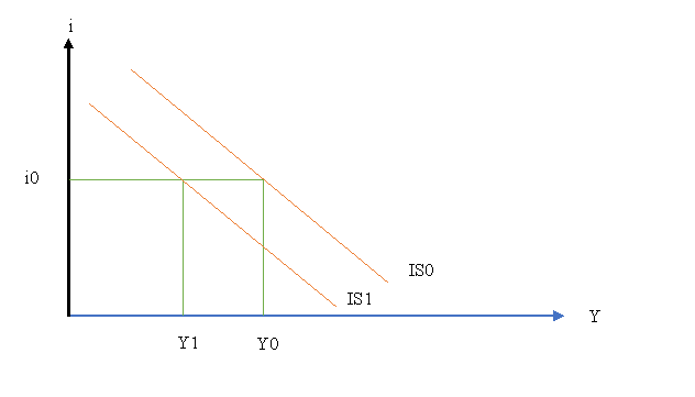
As per the figure above, it can be seen that output has reduced from Y0 to Y1, with the fall in the IS curve from IS0 to IS1.

Now, to explain the situation graphically above figure can be considered. It can be demonstrated through the shifting of the IS curve, up or down or right or left. Now, in order to determine the shift, difference between the savings and investment needs to be considered. If it is assumed that IS curve shifting right, then the output will rise, whereas, interest rate remains same leading to rise in savings. Thus, it will result in higher difference in savings and investment resulting no equilibrium in market. Hence, with the fall in the consumer confidence, IS curve need to shift left. With same interest rate, investment remain constant, however, with fall in the output, there will be fall in the savings (Watanabe 2020). This process will continue, until savings equates with the investment leading to new commodity market equilibrium.

Now, with the fall output and savings, money market ought to change as the disequilibrium in commodity market exists. It will shift the LM curve right wards leading to rise in interest rate to such point, where through increase of the investment and decrease in savings, commodity market achieve equilibrium.

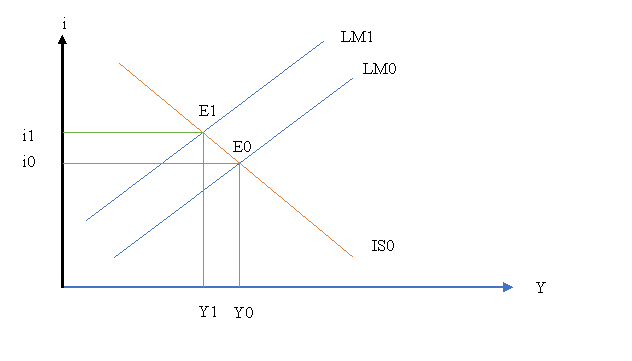
As per the figure above, it can be seen that, initial equilibrium in money market has taken place at E0, where the interest rate is i0 and output is Y0. Now, as the money demand falls, hence, there was shift in the LM curve from LM0 to LM1. This will lead to fall in the demand and higher investment situation resulting rise in interest rate from i0 to i1.

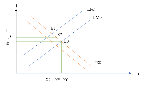
With the shift in the IS curve and LM curve, new market equilibrium will take place, where the output will be Y* and interest rate will be i*. Thus, combining both the IS and LM curve effect, with the fall in consumer demand, as there will be less demand for money and higher investment planning, it will cause in rise of the interest rate and fall in the output.

b.
Consumer confidence is one of the essential factors that influence the money market. Consumer confidence, is an economic indicator that demonstrated the optimism degree that consumers have regarding the overall economic state underpinning their personal financial situation. Considering the consumer confidence, market demand and supply can be changed. For instance, if it is assumed that consumer having higher confidence over the market, it will lead to higher demand in the market in future as consumer will spend more and save less. Thus, the money demand will increase subsequently, leading to lower savings and fall in interest rate. Hence, in money market, higher confidence leads to higher output but lower interest (Andrei et al. 2016). On the other hand, with the fall in consumer confidence, as there will be less demand for money and higher investment planning, it will cause in rise of the interest rate and fall in the output.

To explain the effect of consumer confidence on consumption, investment and private savings, IS-LM model can be used.

Consumption: As the consumer confidence is indicator of the market confidence for the consumers, hence, as there will be change in consumption due to change in the same. For instance, if there is fall in consumer confidence, then people will consume less and save more underpinning the fact that there will be inflation in future (Hayashi and Murphy 2016). However, if it is assumed that the consumer confidence increases, then it will lead to rise in the consumption and lower savings. People then will have higher confidence on market leading to higher consumption.

Investment: As the consumer confidence is indicator of the market confidence for the consumers, hence, as there will be change in consumption due to change in the same. With the lower consumer confidence, private investment will be reduced, however, public investment will be enhanced. On the other hand, with the higher consumer confidence, there will be rise in the private investment, whereas, public investment will fall (Ridha 2016).

Private savings: As the consumer confidence is indicator of the market confidence for the consumers, hence, as there will be change in consumption due to change in the same. If it is assumed that, there is fall in consumer confidence, then the private savings will increase leading to fall in the interest rate in short run. However, with higher consumer confidence, people will save less and consumer more (Fanti Nd Zamparelli 2020).

No, the attempt to save more necessarily will save more is not true. As, with attempt to save more, aggregate demand will fall, there will be less output and this way income will fall and thus, total saving fall in aggregative term. This phenomenon can also be known as paradox of thrift.

c.

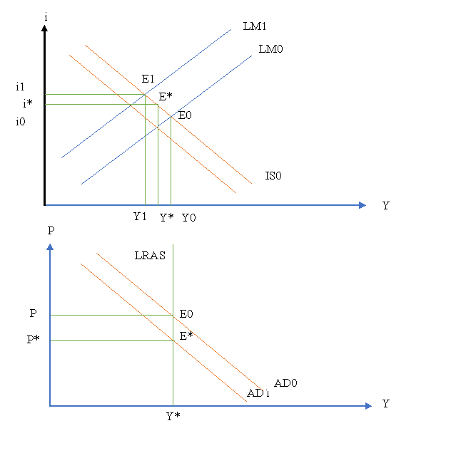
As per the figure above, with the shift in the IS curve and LM curve, new market equilibrium will take place, where the output will be Y* and interest rate will be i*. Thus, combining both the IS and LM curve effect, with the fall in consumer demand, as there will be less demand for money and higher investment planning, it will cause in rise of the interest rate and fall in the output. On the other hand, below figure demonstrates the long run AD-AS situation, where, output and price level is demonstrated. With the fall in the consumer confidence, there will be new market equilibrium at Y*. With the fall in the aggregate demand, AD curve shifts from its initial position of AD0 to AD1. This will lead to fall in price from P to P* in long run.

d.
i.

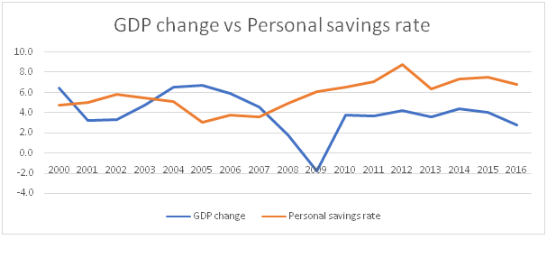
Above figure demonstrates the year over year growth rate of GDP and the Personal saving rate of US. As per the same, it can be seen that there is a negative relation between the GDP growth rate and the personal savings rate. GDP growth rate since 2000 for US has been increased post 2002 after the dotcom crisis. However, personal savings rate since 2002 has started to decrease until 2007, when the Global Financial Crisis came in. Post 2007, as the US economy faced severe crisis, due to GFC, GDP growth rate dipped down to lowest point since Great Depression of 1929. During this time, market confidence was very low, interest rate was high and so does the personal savings rate. This high rate continued until 2012. Post 2009, GDP growth rate increased, however, to with lower market confidence, personal savings rate was also increased. Post 2012, GDP growth rate stabilised for the economy and as market started to have higher confidence, personal saving rate reduced to a substantial level. Underpinning the overall situation, it can be mentioned that there is negative relation between the GDP change and the personal savings rate.

ii.As per the paradox of thrift, savings in aggregate is reduced as the people saves more through the reducing in aggregate demand and output. Figure demonstrated the same situation. As, post 2007, people have lower market confidence, they started to save more and aggregate output reduced. In the successive period, as the output fell and savings continued to increase, however, overall savings started to fall.

Reference:
Andrei, A., Galupa, A., Androniceanu, A. and GEORGESCU, L.I.A., 2016.

MONETARY POLICY WITH CONSTANT REAL STOCK OF BONDS. Economic Computation & Economic Cybernetics Studies & Research, 50(3). Burke, P.J. and Abayasekara, A., 2018. The price elasticity of electricity demand in the United States: A three-dimensional analysis. The Energy Journal, 39(2).
de Rassenfosse, G., 2020. On the price elasticity of demand for trademarks. Industry and Innovation, 27(1-2), pp.11-24.
Denson, C., 2019. Price Elasticity of Demand for Mississippi State University: 2000-2014. Research in Higher Education Journal, 36.
Fanti, L. and Zamparelli, L., 2020. The Paradox of Thrift in the Two-Sector Kaleckian Growth Model.
Fred.stlouisfed.org. 2020. Gross Domestic Product. Economics assignment [online] Available at: https://fred.stlouisfed.org/series/GDP#0 Fred.stlouisfed.org. 2020. Personal Saving Rate. [online] Available at: https://fred.stlouisfed.org/series/PSAVERT

Hayashi, A. and Murphy, D.P., 2017. Savings policy and the paradox of thrift. Yale J. on Reg., 34, p.743. Lima, M.A.F., Carvalho, P.C., Fernández-Ramírez, L.M. and Braga, A.P., 2020. Improving solar forecasting using Deep Learning and Portfolio Theory integration. Energy, 195, p.117016.

Ridha, M.M.B., 2016. The paradox of thrift in an inegalitarian neoclassical economy. Business and Economic Horizons, 12(3), pp.75-93.

Watanabe, T., 2020. Reconsideration of the IS–LM model and limitations of monetary policy: a Tobin–Minsky model. Evolutionary and Institutional Economics Review, pp.1-27.